Measures of Central Tendency

Published

October 8, 2024

1 Background

Collected data possess many observations that we are not interested in each one individually.
Instead, we are interested in summarizing the data in a concise and informative way.
Descriptive measures are single numbers that summarize the data.
They are used to describe the center and spread of the data.
They can be calculated from the data of a sample or a population.
Descriptive measures calculated from the sample are referred to as sample statistics, while those calculated from the population are referred to as population parameters.

2 Measures of central tendency

Measures of central tendency are used to describe the center of the data (i.e., the average or typical value).
They are also referred to as measures of location.
The most common measures of central tendency are the mean, median, and mode.

2.1 Arithmetic Mean

It is calculated by summing all observations and dividing by the total number of observations.
Let $X$ is a random variable:
- The mean of a finite population of size $N$ is denoted by $μ$ , which reads as mu, while the mean of a sample of size $n$ is denoted by $\bar{x}$ , which reads as x-bar.
- The population and sample means can be calculated as follows:
  
  Population mean Sample mean
  
  $μ = \frac{x_{1} + x_{2} + \dots + x_{N}}{N} = \frac{\sum_{i = 1}^{N} x_{i}}{N}$ $\bar{x} = \frac{x_{1} + x_{2} + \dots + x_{n}}{n} = \frac{\sum_{i = 1}^{n} x_{i}}{n}$
Example: consider the variable mpg in the mtcars dataset that we discussed in earlier chapters:
Click to show/hide code
```
mtcars$mpg
```
```
 [1] 21.0 21.0 22.8 21.4 18.7 18.1 14.3 24.4 22.8 19.2 17.8 16.4 17.3 15.2 10.4
[16] 10.4 14.7 32.4 30.4 33.9 21.5 15.5 15.2 13.3 19.2 27.3 26.0 30.4 15.8 19.7
[31] 15.0 21.4
```
- The number of observations can be calculated using the length() function:
  Click to show/hide code
  length(mtcars$mpg)
```
[1] 32
```
- The sum of all values can be calculated using the sum() function:
  Click to show/hide code
  sum(mtcars$mpg)
```
[1] 642.9
```
- $\bar{x} = \frac{21 + 21 + 22.8 + \dots + 21.4}{32} = \frac{642.9}{32} \approx 20.09$
- The mean can be calculated directly using the built-in R function mean():
  Click to show/hide code
  mean(mtcars$mpg)
```
[1] 20.09062
```
  Note
  - If the variable contains missing values, the na.rm argument should be set to TRUE to exclude them before calculating the mean, otherwise, the result will be NA.
  - For example, consider the following variable with some missing values $(1, 2, 3, NA, 5)$ :
    
    Using the mean() function without the na.rm argument will return NA:
    
    Click to show/hide code
    
    x <- c(1, 2, 3, NA, 5) mean(x)
    
    [1] NA
    
    This error can be avoided by setting the na.rm argument to TRUE:
    
    Click to show/hide code
    
    mean(x, na.rm = TRUE)
    
    [1] 2.75
The mean can be calculated if the values are given along with their frequencies as weighted mean:
- Let $x_{1}, x_{2}, \dots, x_{k}$ be the values of a variable with frequencies $f_{1}, f_{2}, \dots, f_{k}$ , then the weighted mean is calculated as:
$\bar{x} = \frac{f_{1} x_{1} + f_{2} x_{2} + \dots + f_{k} x_{k}}{f_{1} + f_{2} + \dots + f_{k}} = \frac{\sum_{i = 1}^{k} f_{i} x_{i}}{\sum_{i = 1}^{k} f_{i}}$
- The weight of each observation $w_{i} = \frac{f_{i}}{\sum_{i = 1}^{k} f_{i}}$ , therefore, the above equation can also be written as $\bar{x} = \sum_{i = 1}^{k} w_{i} x_{i}$
- Example: consider the following variable with values $(1.3, 2.1, 3.5, 4.1, 5.2)$ and frequencies $(2, 3, 1, 4, 2)$ :
  Click to show/hide code
  library(DT) Value = c(1.3, 2.1, 3.5, 4.1, 5.2) Frequency = c(2, 3, 1, 4, 2) my_data <- data.frame( Value, Frequency, Weight = Frequency / sum(Frequency) ) datatable( my_data, options = list( dom = "t", columnDefs = list( list( className = "dt-center", targets = "_all" ) ) ), rownames = FALSE )
  Value Frequency Weight
  
  1.3 2 0.1666666666666667
  2.1 3 0.25
  3.5 1 0.08333333333333333
  4.1 4 0.3333333333333333
  5.2 2 0.1666666666666667
  - The weighted mean is calculated as:
  $\bar{x} = \frac{2 \times 1.3 + 3 \times 2.1 + 1 \times 3.5 + 4 \times 4.1 + 2 \times 5.2}{2 + 3 + 1 + 4 + 2} =$
  
  $\frac{2.6 + 6.3 + 3.5 + 16.4 + 10.4}{12} = \frac{39.2}{12} \approx 3.27$
  - It can also be calculated using the weights as follows:
    Click to show/hide code
    
    with(my_data, sum(Value * Weight))
    [1] 3.266667
  - The built-in R function weighted.mean() can be used for direct calculation:
    Click to show/hide code
    
    weighted.mean( x = my_data$Value, w = my_data$Frequency) # w represents the weights which can be given as frequencies or weights
    [1] 3.266667

Population mean	Sample mean
$μ = \frac{x_{1} + x_{2} + \dots + x_{N}}{N} = \frac{\sum_{i = 1}^{N} x_{i}}{N}$	$\bar{x} = \frac{x_{1} + x_{2} + \dots + x_{n}}{n} = \frac{\sum_{i = 1}^{n} x_{i}}{n}$

Value	Frequency	Weight
1.3	2	0.1666666666666667
2.1	3	0.25
3.5	1	0.08333333333333333
4.1	4	0.3333333333333333
5.2	2	0.1666666666666667

2.1.1 Characteristics of the mean

The sum of deviations of the observations from the arithmetic mean is always zero:

$\sum_{i = 1}^{n} (x_{i} - \bar{x}) = 0$

The sum of the squared deviations of the observations from a certain value is the least (i.e., minimized) when this value is the mean (this is referred to as the least squares principle).
If a constant $c$ is added to each observation, the mean is also increased by $c$ , i.e., the mean of $x_{i} + c = \bar{x} + c$ .
If the observations are multiplied by a constant $c$ , then the mean is also multiplied by $c$ , i.e., the mean of $c x_{i} = c \bar{x}$ .
If the observations $x_{1}, x_{2}, \dots x_{n}$ are linearly transformed, where $y_{i} = a + b x_{i}$ ( $a$ and $b$ are known constants), then it holds that $\bar{y} = a + b \bar{x}$ .
The mean is sensitive to extreme values (outliers), and it may not be a good measure of central tendency in the presence of outliers.
Listing 1: Impact of outliers on the mean
- Example: consider the following variable with values $(32.1, 34.5, 33.6, 37.2, 39.4)$ the mean is calculated as follows:
  
  Click to show/hide code
  
  x <- c(32.1, 34.5, 33.6, 37.2, 39.4) mean(x)
  
  [1] 35.36
  
  Lets replace the last value with an extreme value of $250.1$ , so the values would be:
  
  Click to show/hide code
  
  x[5] <- 250.1 x
  
  [1] 32.1 34.5 33.6 37.2 250.1
  
  The mean of the new values with the outlier would be:
  
  Click to show/hide code
  
  mean(x)
  
  [1] 77.5
  
  The presence of the outlier affected the mean that it is no longer a good measure of central tendency for this variable.

2.2 Median

The median, denoted by ${\tilde{x}}_{0.5}$ , is the value which divides the ordered observations into two equal parts (i.e., at least 50% of the values $\geq$ the median and at least 50% of the values $\leq$ the median).
The median is calculated as follows:
- If the number of observations is odd, the median is the middle value of the ordered observations.
- If the number of observations is even, the median is the arithmetic mean of the two middle observations.

${\tilde{x}}_{0.5} = {\begin{cases} x_{\frac{n + 1}{2}} & if n is odd \\ \frac{1}{2} (x_{\frac{n}{2}} + x_{\frac{n}{2} + 1}) & if n is even \end{cases}$

Example B.3.1
Example B.3.2

Consider the following set of observations: $(3, 5, 7, 7, 7, 9, 11)$ .
- There is an odd number of observations $n = 7$ , so the median is the middle value of the ordered observations, which is ranked $\frac{n + 1}{2} = \frac{7 + 1}{2} = 4^{t h}$ and its value is $7$ .
- Half of the measurements $(3, 5, 7)$ are below or equal to $7$ , and half of the measurements $(7, 9, 11)$ are equal to or above $7$ .
- Therefore, the previous defintion of the median contains “equal to” to cover the case of having repeated, similar values.

Example: the variable mpg has $32$ observations, so the median is the arithmetic mean of the two middle observations (i.e., the mean of the ordered observations ranked $\frac{32}{2} = 16^{t h}$ and $\frac{32}{2} + 1 = 17^{t h}$ ):
- The ordered observations are:
  Click to show/hide code
  mpg_ordered <- sort(mtcars$mpg) mpg_ordered
```
 [1] 10.4 10.4 13.3 14.3 14.7 15.0 15.2 15.2 15.5 15.8 16.4 17.3 17.8 18.1 18.7
[16] 19.2 19.2 19.7 21.0 21.0 21.4 21.4 21.5 22.8 22.8 24.4 26.0 27.3 30.4 30.4
[31] 32.4 33.9
```
- The $16^{t h}$ and $17^{t h}$ ordered observations are:
  Click to show/hide code
  mpg_ordered[16:17]
```
[1] 19.2 19.2
```
- The median is the arithmetic mean of these two values:
  Click to show/hide code
  mean(mpg_ordered[16:17])
```
[1] 19.2
```
- The median can also be calculated using the built-in R function median():
  Click to show/hide code
  median(mtcars$mpg)
```
[1] 19.2
```

2.2.1 Characteristics of the median

Unlike the mean, the median is not drastically affected by extreme values (outliers).
Consider the example discussed above Listing 1:
- The median of the original set of observations is:
  Click to show/hide code
  median(c(32.1, 34.5, 33.6, 37.2, 39.4))
```
[1] 34.5
```
- The median of the set of observations with the outlier is:
  Click to show/hide code
  median(c(32.1, 34.5, 33.6, 37.2, 250.1))
```
[1] 34.5
```
- Because the median is concerned with the middle value, it is less affected by the presence of the outliers than the mean.
The median is a robust measure of central tendency, and it is preferred when the data is skewed or contains outliers.

2.3 Quantiles

Quantiles are a generalization of of the concept of the median.
A quantile is defined as the value that divides the ordered observations into two parts such that a certain proportion of the observations are less than or equal to the quantile.
In this sense, the median is the $50^{t h}$ quantile because at least $50 %$ of the observations are less than or equal to the median.
Similarly, the $20^{t h}$ quantile is the value that divides the ordered observations into two parts such that at least $20 %$ of the observations are less than or equal to the that quantile, while at least $80 %$ of the observations are greater than or equal to that quantile.

General definition of quantiles

Let $α$ be a number between $0$ and $1$ .
The $[(α \times 100) %$ quantile is denoted by ${\tilde{x}}_{α}$ .
It is defined as the value that splits the data into two parts such that at least $α \times 100 %$ of the observations are less than or equal to the quantile, while at least $(1 - α) \times 100 %$ of the observations are greater than or equal to the quantile.

Deciles divide the data into $10$ parts, corresponding to quantiles at $α = 0.1, 0.2, \dots, 0.9$ .
Quintiles divide the data into $5$ parts, corresponding to quantiles at $α = 0.2, 0.4, 0.6, 0.8$ .
Quartiles divide the data into $4$ parts, corresponding to quantiles at $α = 0.25, 0.5, 0.75$ .
Percentiles: if $(α \times 100)$ takes an integer value, the quantile is referred to as a percentile (i.e, divide the data into $100$ equal parts).

2.3.1 Calculation of quantiles

The quantiles can be obtained in R using the quantile() function.
For example, the quantiles of the variable mpg in the mtcars dataset can be calculated as follows:
Click to show/hide code
```
quantile(mtcars$mpg)
```
```
    0%    25%    50%    75%   100% 
10.400 15.425 19.200 22.800 33.900 
```
By default, The function outputs the $0^{t h}$ , $25^{t h}$ , $50^{t h}$ , $75^{t h}$ , and $100^{t h}$ quantiles (i.e., the minimum, first quartile, median, third quartile, and maximum).
To get a specific quantile, use the probs argument to add a vector of the desired probabilities (i.e., $α$ ). For example, the following code can be used to get the $5^{t h}$ and $95^{t h}$ quantiles:
Click to show/hide code
```
quantile(
  mtcars$mpg, 
  probs = c(0.05, 0.95)
)
```
```
    5%    95% 
11.995 31.300 
```
R provides nine algorithms to calculate the quantiles, which can be specified using the type argument:
- Types $1 - 3$ are used for discontinuous data, while types $4 - 9$ are used for continuous data.
- Type $1$ and $3$ are used for class “Date” and for ordered factors.
- Type $7$ is the default method for continous data.
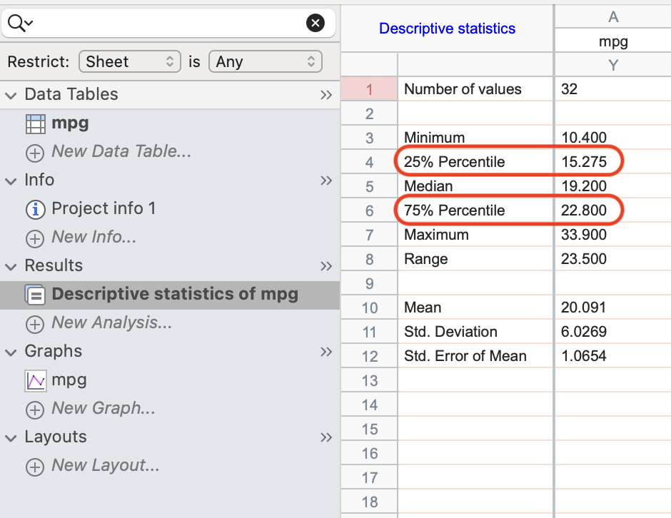
- Type $6$ is used to get results similar to SPSS, Minitab, or Graphpad Prism.
- For example, the of $25^{t h}$ and $75^{t h}$ quantiles of the variable mpg in the mtcars dataset using R (type $6$ or $7$ ), SPSS, and, Graphpad Prism are as follows:
  Using type $6$ :
  
  Click to show/hide code
  
  quantile( mtcars$mpg, probs = c(0.25, 0.75), type = 6 )
  
  25% 75% 15.275 22.800
  
  Using type $7$ :
  
  Click to show/hide code
  
  quantile( mtcars$mpg, probs = c(0.25, 0.75), type = 7 )
  
  25% 75% 15.425 22.800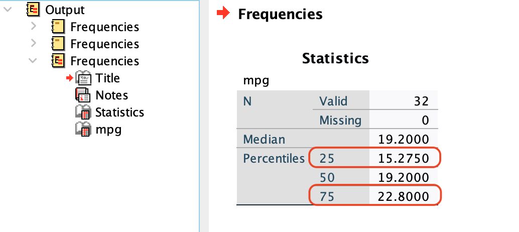
- Detailed discussion of the algorithms used to calculate the quantiles can be found here.

2.4 Trimean

The trimean is defined as weighted average of the first quartile $(Q_{1})$ , the median $(Q_{2})$ , and the third quartile $(Q_{3})$ :

$Trimean = \frac{Q_{1} + (2 \times Q_{2}) + Q_{3}}{4}$

The trimean is a robust measure of central tendency and has the advantage that it uses more information than the median, which is based on only one value and ignores the overall distribution.

2.5 Mode

The mode of a set of observations is the observation that occurs most frequently compared with all other values.
A set of observations can have:
- No mode (if all observations occur with the same frequency).
- One mode (if one observation occurs most frequently).
- More than one mode (if two or more observations occur with the same highest frequency).
Example: consider the variable cyl (number of car cylinders) in the mtcars dataset:
- R has no direct built-in function to calculate the mode, but it can be calculated from the frequency table as follows:
  Click to show/hide code
  library(dplyr) # create table of the frequencies of the values freq_tbl <- table(mtcars$cyl) # convert to adata frame freq_df <- as.data.frame(freq_tbl) names(freq_df)[1] <- "cyl" # arrange the values in descending order of frequency freq_df <- freq_df %>% arrange(desc(Freq)) freq_df
```
  cyl Freq
1   8   14
2   4   11
3   6    7
```
  Click to show/hide code
  paste( "The mode is", freq_df$cyl[which.max(freq_df$Freq)], "cyliners" )
```
[1] "The mode is 8 cyliners"
```
- The mode can also be calculated directly using the Mode() function from the DescTools package:
  Click to show/hide code
  library(DescTools)
```
Warning: package 'DescTools' was built under R version 4.4.1
```
  Click to show/hide code
  Mode(mtcars$cyl)
```
[1] 8
attr(,"freq")
[1] 14
```
  - The first line of the output shows the mode ( $8$ cylinders) and the last line shows the frequency of the mode.
Caution
- R has a built-in function mode() that returns the storage mode of an object (e.g., numeric, character, etc.) rather than the mode.
  Click to show/hide code
  
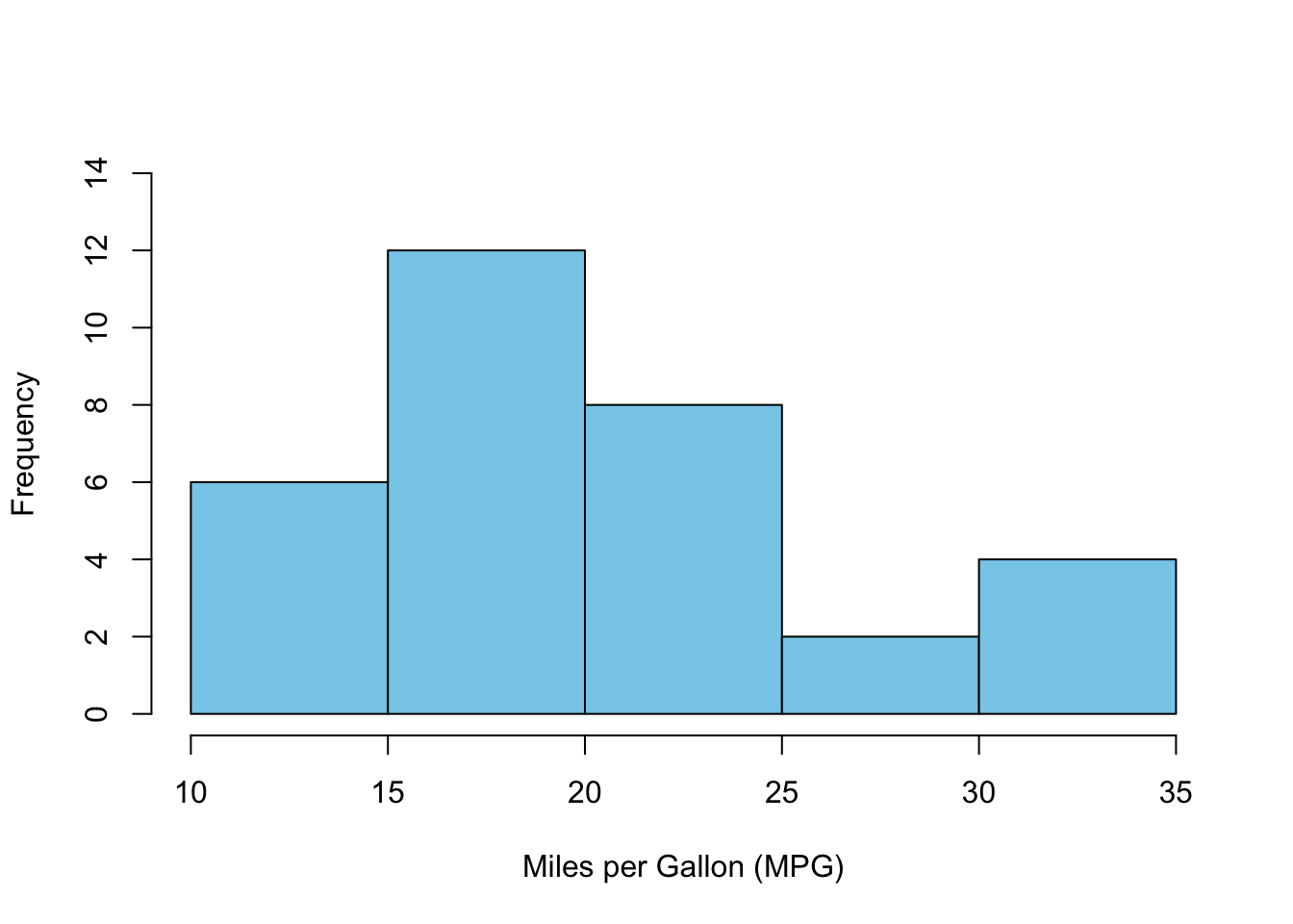
  mode(mtcars$cyl)
  
  [1] "numeric"
- For numerical data which contains many unique values, the mode may not be a good measure of central tendency. However, if the observations are summarized in groups (e.g., frequency table or histogram), the mode can be calculated as the class interval with the highest frequency.
  - Example: consider the histogram of the variable mpg in the mtcars dataset:
    - The class interval $(15, 20]$ has the highest frequency of $12$ observations, so the mode is the interval $(15, 20]$ (others may also consider the midpoint of the interval, $17.5$ , as the mode).

2.6 Geometric mean

Let $X$ a quantitative random variable with positive and non-zero values $x_{1}, x_{2}, \dots, x_{n}$ , then the geometric mean $({\bar{x}}_{G})$ is computed by multiplying all the values and then taking the $n^{t h}$ root of the product:

${\bar{x}}_{G} = \sqrt[n]{x_{1} \times x_{2} \times \dots \times x_{n}} = {(\prod_{i = 1}^{n} x_{i})}^{\frac{1}{n}}$
It is less sensitive to extreme values in skewed distributions than the arithmetic mean.
Geometric mean is used for averaging data that are multiplicative in nature (e.g., percentage change and rates).
- Percentage change is calculated as the difference between the final $(x_{1})$ and initial $(x_{0})$ values divided by the initial value, then multiplied by $100$ :
  
  $Percentage change = (\frac{x_{1} - x_{0}}{x_{0}}) \times 100$
  - If the sign of the percentage change is positive, it indicates an increase, while a negative sign indicates a decrease.
- Rate is the ratio of two quantities that describes how one quantity changes with respect to another (e.g., speed, growth rate, and interest rate).

Consider the following set of observations: $(4, 16, 64, 256)$ .
The geometric mean is calculated as:

$\sqrt[4]{4 \times 16 \times 64 \times 256} = \sqrt[4]{1048576} = 32$
The geometric mean can be calculated using the Gmean() function from the DescTools package or the geometric.mean() function from the psych package:
Click to show/hide code
```
library(DescTools)
library(psych)
x <- c(4, 16, 64, 256)
Gmean(x)
```
```
[1] 32
```
Click to show/hide code
```
geometric.mean(x)
```
```
[1] 32
```

Assume a bank provides the following interest rates for a three-year plan: $3.3 %$ in the first year, $4.5 %$ in the second year, and $5.2 %$ in the third year.

If a client deposits $$ 500$ , the change in the amount can be calculated as follows:

Time	Year	Amount $($)$	Rate $(%)$	Interest $($)$ $({Rate}_{t} \times {Amount}_{t - 1})$	Growth factor $({Amount}_{t} / {Amount}_{t - 1})$
$t_{0}$	0	$500.0$	–	–	–
$t_{1}$	1	$516.5$	$3.3$	$16.5$	$1.033$
$t_{2}$	2	$539.7$	$4.5$	$23.2$	$1.045$
$t_{3}$	3	$567.8$	$5.2$	$28.1$	$1.052$

The interest rate is also known as the growth rate.
The growth rate $= (growth factor - 1) \times 100$ .
The average growth factor is calculated as the geometric mean of the growth factors:
Click to show/hide code
```
growth_factors <- c(1.033, 1.045, 1.052)
Gmean(growth_factors)
```
```
[1] 1.043304
```
So, the average growth rate per year $= (1.043 - 1) \times 100 = 4.3 %$ .
This average growth rate can also be obtained by calculating the geometric mean of the interest (growth) rates:
Click to show/hide code
```
interest_rates <- c(3.3, 4.5, 5.2)
Gmean(interest_rates)
```
```
[1] 4.258369
```
However, this approach is not recommended because the interest rates can be negative (the rate decreases), which results in error while computing the geometric mean.
The total amount of money ( $A$ ) can be calculated at any year using the formula: $A_{t} = A_{t_{0}} \times (average growth factor)^{t}$ . For example, the amount at the end of the third year $= 500 \times {1.043304}^{3} = $ 567.8$ .

Calculate the average interest rate for the following four-year plan: $10 %$ , $14 %$ , $15 %$ , and $- 5 %$ .

The average rate per year is $%$ (to one decimal place)

The average interest rate can not be computed directly by calculating the geometric mean of the interest rates because the last rate is negative.
Therefore, we calculate the average growth factor as the geometric mean of the growth factors.
Growth factor $= \frac{rate}{100} + 1$
So, the growth factors are $(1.1, 1.14, 1.15, 0.95)$ .

The average growth factor is equal to:

Click to show/hide code

growth_factors <- c(1.1, 1.14, 1.15, 0.95)
Gmean(growth_factors)

[1] 1.081882

Therefore, the average interest rate per year is $8.2 %$ .

2.6.1 Geometric mean and logarihmic transformation

If the observations are transformed by taking the logarithm (common or natural), the antilogarithm of the arithmetic mean of the transformed values is equal to the geometric mean of the original values.
- Let $X$ be a random variable with positive, non-zero values $x_{1}, x_{2}, \dots, x_{n}$ , and $Y$ is the transformed variable with values $y_{1}, y_{2}, \dots, y_{n}$ such that $y_{i} = \log_{10} (x_{i})$ :
- The arithmetic mean of the transformed values is calculated as:
$\bar{y} = \frac{y_{1} + y_{2} + \dots + y_{n}}{n} = \frac{\log_{10} (x_{1}) + \log_{10} (x_{2}) + \dots + \log_{10} (x_{n})}{n} =$

$\log_{10} (\sqrt[n]{x_{1} \times x_{2} \times \dots \times x_{n}})$
- The antilogarithm of the arithmetic mean of the transformed values is:
$10^{\bar{y}} = 10^{\log_{10} (\sqrt[n]{x_{1} \times x_{2} \times \dots \times x_{n}})} = \sqrt[n]{x_{1} \times x_{2} \times \dots \times x_{n}}$
- The last equation represents the geometric mean of the original values.
Example: consider the following set of observations $(5, 9, 10, 22, 13, 50)$ , the following table shows the original and $l o g_{10}$ transformed values:
Click to show/hide code

library(DT) x <- c(5, 9, 10, 22, 13, 50) y <- round(log10(x), 5) my_data <- data.frame( Original = x, Log10_transformed = y ) datatable( my_data, options = list( dom = "t", columnDefs = list( list( className = "dt-center", targets = "_all" ) ) ), rownames = FALSE )
Original Log10_transformed

5 0.69897
9 0.95424
10 1
22 1.34242
13 1.11394
50 1.69897
- The arithmetic mean of the transformed values is:
  Click to show/hide code
  mean(y)
```
[1] 1.134757
```
- The antilogarithm of the arithmetic mean of the transformed values is:
  Click to show/hide code
  10^mean(y)
```
[1] 13.63819
```
- The geometric mean of the original values is:
  Click to show/hide code
  Gmean(x)
```
[1] 13.63823
```
- The antilogarithm of the arithmetic mean of the transformed values is equal to the geometric mean of the original values.
Note
- When the original values are log transformed, the back-transformed mean is not the same as the original mean but it is the geometric mean of the original values.
- On the other hand, back-transforming the median of the log-transformed values gives the median of the original values:
  - For the mpg variable from the mtcars dataset, the median of the log-transformed values is:
    
    Click to show/hide code
    
    med_log <- median( log(mtcars$mpg)) med_log
    
    [1] 2.95491
  - The antilogarithm of the median (back transformation) of the log-transformed values is:
    
    Click to show/hide code
    
    exp(med_log) # exponentiation to back transform
    
    [1] 19.2
  - The median of the original values is:
    
    Click to show/hide code
    
    median(mtcars$mpg)
    
    [1] 19.2
  - The antilogarithm of the median of the log-transformed values is equal to the median of the original values.

Original	Log10_transformed
5	0.69897
9	0.95424
10	1
22	1.34242
13	1.11394
50	1.69897

2.7 Harmonic mean

The harmonic mean $({\bar{x}}_{H})$ is the reciprocal of the arithmetic mean of the reciprocals of the observations:
- Let $X$ be a random variable with values $x_{1}, x_{2}, \dots, x_{n}$ , then the reciprocals of the observations are $\frac{1}{x_{1}}, \frac{1}{x_{2}}, \dots, \frac{1}{x_{n}}$ , and their arithmetic mean is calculated as:
$\frac{1}{n} (\frac{1}{x_{1}} + \frac{1}{x_{2}} + \dots + \frac{1}{x_{n}}) = \frac{\sum_{i = 1}^{n} \frac{1}{x_{i}}}{n}$
- The harmonic mean is the reciprocal of the arithmetic mean of the reciprocals:
${\bar{x}}_{H} = \frac{n}{\sum_{i = 1}^{n} \frac{1}{x_{i}}}$
It is used for averaging data that are ratios or rates (e.g., speed or financial ratios).
If the observations do not contribute equally towards the calculation of the mean (i.e., the observations have different weights), the harmonic mean can be weighted:
- Let $X$ be a random variable with values $x_{1}, x_{2}, \dots, x_{n}$ that have coressponding weights $w_{1}, w_{2}, \dots, w_{n}$ , then the harmonic mean is calculated as:
$Weighted {\bar{x}}_{H} = \frac{w_{1} + w_{2} + \dots + w_{n}}{\frac{w_{1}}{x_{1}} + \frac{w_{2}}{x_{2}} + \dots + \frac{w_{n}}{x_{n}}} = \frac{\sum_{i = 1}^{n} w_{i}}{\sum_{i = 1}^{n} \frac{w_{i}}{x_{i}}} = \frac{1}{\sum_{i = 1}^{n} \frac{w_{i}}{x_{i}}}$
Example: consider the following set of observations $(2, 4, 6, 8)$ :
- The harmonic mean is calculated as:
  Click to show/hide code
  x <- c(2, 4, 6, 8) n <- length(x) harmonic_mean <- n / sum(1 / x) harmonic_mean
```
[1] 3.84
```
- The harmonic mean can also be calculated using the Hmean() function from the DescTools package or harmonic.mean() function from the psych package:
  Click to show/hide code
  library(DescTools) Hmean(x)
```
[1] 3.84
```
  Click to show/hide code
  library(psych) harmonic.mean(x)
```
[1] 3.84
```
The harmonic mean is used to calculate some statistical measures such as F1 score used to assess the performance of logistic regression models. In addition, it is used during pairwise multiple comparisons.

Example B.3.5
Example B.3.6

A car travels $100 km$ at a speed $60 km/h$ , $100 km$ at $70 km/h$ , $100 km$ at $90 km/h$ , and $100 km$ at $100 km/h$ . Calculate the average speed of the car.

The arithmetic mean of the speed $= \frac{60 + 70 + 90 + 100}{4} = \frac{320}{4} = 80$ km/h.
However, this method ignores the time taken to travel each distance.
The time taken to travel each distance is given in the following table:

Speed (km/h)	Distanc (km)	Time (h) [Distance/Speed]
$60$	$100$	$1.666667$
$70$	$100$	$1.428571$
$90$	$100$	$1.111111$
$100$	$100$	$1$

The total distance traveled is $400$ km, and the total time taken is $5.21 h$ So, the actual average speed $= \frac{400}{5.206349} \approx 76.83 km/h$ .
This average can be found using the harmonic mean of the speeds:
Click to show/hide code
```
speeds <- c(60, 70, 90, 100)
Hmean(speeds)
```
```
[1] 76.82927
```
The average speed can also be calculated as the weighted arithmetic mean using weights based on the time taken to travel each distance:
Click to show/hide code
```
times <- c(100/60, 100/70, 100/90, 100/100) # use times as weights
weighted.mean(speeds, w = times)
```
```
[1] 76.82927
```

Note

To find the average of rates with different numerators but the same denominator use the arithmetic mean or weighted harmonic mean (weights are based on numerators).
To find the average of rates with same numerators but different denominators use the harmonic mean or weighted arithmetic mean (weights are based on denominators).
To find the average of rates with different numerators and denominators use the weighted arithmetic mean (weights are based on denominators) or weighted harmonic mean (weights are based on numerators).

Suppose that you invested $$ 2550$ in stock market. In the first year, you spent $$ 1000$ to purchase $40$ shares of stock $A$ . In the second year, you spent $$ 1550$ to purchase $78$ shares of the same stock. Calculate the average price per share.

The rate here is the price $($)$ per share.
The total amount of the shares bought $= 40 + 78 = 118$ shares, so the actual average price per share $= \frac{2550}{118} \approx $ 21.61$ .
In the first year, the price per share $= \frac{1000}{40} = $ 25$ .
In the second year, the price per share $= \frac{1550}{78} \approx $ 19.87$ .

Year	Price per share $($ / share)$	Amount invested $($)$	Number of shares
$1$	$25.00$	$1000$	$40$
$2$	$19.87$	$1550$	$78$

The arithmetic mean of the price per share $= \frac{25 + 19.87}{2} = \frac{44.87}{2} = $ 22.44$ , which is higher than the actual average price per share.
Because both the numerator (amount invested) and denominator (number of shares) are different, the weighted arithmetic or weighted harmonic mean should be used to calculate the average price per share:
- The weighted arithmetic mean using denominator (number of shares) as weights:
  Click to show/hide code
  weights_1 <- c(40/118, 78/118) price_1 <- 1000/40 price_2 <- 1550/78 weighted.mean(c(price_1, price_2), w = weights_1)
```
[1] 21.61017
```
- The weighted harmonic mean using numerators (amount invested) as weights:
  Click to show/hide code
  weights_2 <- c(1000/2550, 1550/2550) h_mean <- 1/sum(weights_2 / c(price_1, price_2)) h_mean
```
[1] 21.61017
```

2.8 Trimmed mean

The observations are arranged based on magnitude, then a certain percentage of the observations are removed from both ends of the ordered observations.
The trimmed mean $({\bar{x}}_{T})$ is then calculated as the arithmetic mean of the remaining observations.
Typically, $5 %$ to $25 %$ of the observations are trimmed from each end.
The trimmed mean is less sensitive to outliers than the arithmetic mean becuase the extreme values are removed.
Some robust statistical tests use the trimmed mean such as Yuen’s test, which is used to compare the trimmed means of two groups when the assumption of normality is violated.
Trimmed mean can be calculated in R using the mean() function with the trim argument set to the percentage of observations to be trimmed.
- Example: the $5 %$ trimmed mean of the variable mpg in the mtcars dataset is calculated as follows:
  Click to show/hide code
  mean(mtcars$mpg, trim = 0.05)
```
[1] 19.95333
```
  - DescTools package has a function Trim() that is an excerpt from the base function mean() but returns the trimmed data without calculating the mean:
    Click to show/hide code
    
    library(DescTools) mpg_ordered <- sort(mtcars$mpg) Trim(mpg_ordered, 0.05)
    [1] 10.4 13.3 14.3 14.7 15.0 15.2 15.2 15.5 15.8 16.4 17.3 17.8 18.1 18.7 19.2 [16] 19.2 19.7 21.0 21.0 21.4 21.4 21.5 22.8 22.8 24.4 26.0 27.3 30.4 30.4 32.4 attr(,"trim") [1] 1 32
    - The output shows the cleaned data after trimming $5 %$ of the observations from each end and the location of the trimmed observations (the $1^{st}$ and $32^{nd}$ observations that were removed).
    - The percentage of trimming is multiplied by the number of observations to get the number of observations to be trimmed from each end (i.e., $0.05 \times 32 = 1.6$ observations, which R rounds down to $1$ ).
    - Therefore, one observation has been removed from each end.
$50 %$ trimming is equivalent to the median:
Click to show/hide code
```
mean(mtcars$mpg, trim = 0.5)
```
```
[1] 19.2
```
Discarding the extreme values leads to loss of information that can introduce bias in the estimation of the mean. Therefore, trimming should be used cautiously. It can be safely used to discard extreme values (outliers) that might be due to errors during measurement or data collection or when the extreme values are irrelevant to the rest of the data.

2.9 Winsorized mean

The observations are arranged based on magnitude, then the extreme values beyond a certain percentile threshold are replaced by these threshold values.
For example, $5 %$ Winsorization involves replacing the values smaller than the $5^{t h}$ percentile with the $5^{t h}$ percentile value and the values larger than the $95^{t h}$ percentile with the $95^{t h}$ percentile value.
The Winsorized mean $({\bar{x}}_{W})$ is then calculated as the arithmetic mean of the modified observations.
The Winsorized mean is less sensitive to outliers than the arithmetic mean.
To Winsorize data, the Winsorize() function from the DescTools package can be used:
- The function has probs argument that takes a vector of two values representing the lower and upper percentiles to be Winsorized (e.g., probs = c(0.05, 0.95) for $5 %$ Winsorization).
- In addition, there is type argument that specifies the algorithm to be used for calculating the perecentiles (discussed in details here).
- Example: the variable mpg in the mtcars dataset is $5 %$ Winsorized as follows:
  - Calculate the $5^{t h}$ and $95^{t h}$ percentiles of the variable mpg:
    Click to show/hide code
    
    quantile( mtcars$mpg, probs = c(0.05, 0.95), type = 7 )
    5% 95% 11.995 31.300
  - The quantile() function has been used to calculate the $5^{t h}$ and $95^{t h}$ percentiles of the variable mpg, which are $11.995$ and $31.3$ , respectively. The type argument is set to $7$ , which is the default algorithm for calculating the percentiles in R for continuous data.
  - Display the original values in order:
    Click to show/hide code
    
    mpg_ordered
    [1] 10.4 10.4 13.3 14.3 14.7 15.0 15.2 15.2 15.5 15.8 16.4 17.3 17.8 18.1 18.7 [16] 19.2 19.2 19.7 21.0 21.0 21.4 21.4 21.5 22.8 22.8 24.4 26.0 27.3 30.4 30.4 [31] 32.4 33.9
  - Winsorize the variable mpg using the $5^{t h}$ and $95^{t h}$ percentiles:
    Click to show/hide code
    
    library(DescTools) mpg_win <- Winsorize( x = mpg_ordered, val = quantile( mpg_ordered, probs = c(0.05, .95) ) ) mpg_win
    [1] 11.995 11.995 13.300 14.300 14.700 15.000 15.200 15.200 15.500 15.800 [11] 16.400 17.300 17.800 18.100 18.700 19.200 19.200 19.700 21.000 21.000 [21] 21.400 21.400 21.500 22.800 22.800 24.400 26.000 27.300 30.400 30.400 [31] 31.300 31.300
  - The output of the Winsorize() function shows that the two smallest values $(10.4 and 10.4)$ that are smaller than the $5^{t h}$ percentile $(11.995)$ have been replaced by the $5^{t h}$ percentile. Whereas, the two largest values $32.4 and 33.9$ that are larger than the $95^{t h}$ percentile $(31.3)$ have been replaced by the $95^{t h}$ percentile.
  - Calculate the Winsorized mean of the variable mpg:
    Click to show/hide code
    
    mean(mpg_win)
    [1] 20.07469
  - The Winsorized mean can be calculated directly using the function winsor.mean() function from the psych package:
    Click to show/hide code
    
    library(psych) winsor.mean( mtcars$mpg, trim = 0.05 )
    [1] 20.07469
Unlike trimming, Winsorization preserves some of the original information in the data. The extreme values are not totally discarded but their weight (impact) is reduced.

3 References

Daniel, W. W. and Cross, C. L. (2013). Biostatistics: A Foundation for Analysis in the Health Sciences, Tenth edition. Wiley
Heumann, C., Schomaker, M., and Shalabh (2022). Introduction to Statistics and Data Analysis: With Exercises, Solutions and Applications in R. Springer
Hoffman, J. (2019). Basic Biostatistics for Medical and Biomedical Practitioners, Second Edition. Academic Press
Lane, D. M. et al., (2019). Introduction to Statistics. Online Edition. Retrieved September 14, 2024, from https://openstax.org/details/introduction-statistics